CellRank Meets Experimental Time
Preliminaries
In this tutorial, you will learn how to:
match cells across experimental time points using a
TemporalProblem[].set up a
RealTimeKernelto combine transitions within- and across time-points.visualize these transitions in a low dimensional embedding.
This tutorial notebook can be downloaded using the following link.

The Moscot/CellRank interface: Any type of temporal moscot problem, including the TemporalProblem, the LineageProblem (see moslin) and the SpatioTemporalProblem, can be passed to CellRank for further analysis [].
Note
If you want to run this on your own data, you will need:
a scRNA-seq dataset with experimental time points. Additional spatial or lineage information improves the accuracy of fate mapping, but is not required.
Note
If you encounter any bugs in the code, our if you have suggestions for new features, please open an issue. If you have a general question or something you would like to discuss with us, please post on the scverse discourse.
Import packages & data
%load_ext autoreload
%autoreload 2
import sys

if "google.colab" in sys.modules:
    !pip install -q git+https://github.com/scverse/cellrank
import cellrank as cr
import scanpy as sc
import session_info2
from cellrank.kernels import RealTimeKernel
from moscot.problems.time import TemporalProblem

sc.set_figure_params(frameon=False, dpi=100)
cr.settings.logging_level = "INFO"
import warnings

warnings.simplefilter("ignore", category=UserWarning)
To demonstrate the appproach in this tutorial, we will use a scRNA-seq dataset of MEF reprogramming , which can be conveniently acessed through reprogramming_schiebinger.
adata = cr.datasets.reprogramming_schiebinger(subset_to_serum=True)
adata
AnnData object with n_obs × n_vars = 165892 × 19089
    obs: 'day', 'MEF.identity', 'Pluripotency', 'Cell.cycle', 'ER.stress', 'Epithelial.identity', 'ECM.rearrangement', 'Apoptosis', 'SASP', 'Neural.identity', 'Placental.identity', 'X.reactivation', 'XEN', 'Trophoblast', 'Trophoblast progenitors', 'Spiral Artery Trophpblast Giant Cells', 'Spongiotrophoblasts', 'Oligodendrocyte precursor cells (OPC)', 'Astrocytes', 'Cortical Neurons', 'RadialGlia-Id3', 'RadialGlia-Gdf10', 'RadialGlia-Neurog2', 'Long-term MEFs', 'Embryonic mesenchyme', 'Cxcl12 co-expressed', 'Ifitm1 co-expressed', 'Matn4 co-expressed', '2-cell', '4-cell', '8-cell', '16-cell', '32-cell', 'cell_growth_rate', 'serum', '2i', 'major_cell_sets', 'cell_sets', 'batch'
    var: 'highly_variable', 'TF'
    uns: 'batch_colors', 'cell_sets_colors', 'day_colors', 'major_cell_sets_colors'
    obsm: 'X_force_directed'
    obsp: 'transition_matrix'
Massage the time point annotations.
adata.obs["day"] = adata.obs["day"].astype(float).astype("category")

# In addition, it's nicer for plotting to have numerical values.
adata.obs["day_numerical"] = adata.obs["day"].astype(float)
Subsample to speed up the analysis - this tutorial is meant to run in a couple of minutes on a laptop. It’s not a problem for CellRank to do any of the computations here on the full data, we’d just have to wait a bit longer.
sc.pp.subsample(adata, fraction=0.25, random_state=0)
adata
AnnData object with n_obs × n_vars = 41473 × 19089
    obs: 'day', 'MEF.identity', 'Pluripotency', 'Cell.cycle', 'ER.stress', 'Epithelial.identity', 'ECM.rearrangement', 'Apoptosis', 'SASP', 'Neural.identity', 'Placental.identity', 'X.reactivation', 'XEN', 'Trophoblast', 'Trophoblast progenitors', 'Spiral Artery Trophpblast Giant Cells', 'Spongiotrophoblasts', 'Oligodendrocyte precursor cells (OPC)', 'Astrocytes', 'Cortical Neurons', 'RadialGlia-Id3', 'RadialGlia-Gdf10', 'RadialGlia-Neurog2', 'Long-term MEFs', 'Embryonic mesenchyme', 'Cxcl12 co-expressed', 'Ifitm1 co-expressed', 'Matn4 co-expressed', '2-cell', '4-cell', '8-cell', '16-cell', '32-cell', 'cell_growth_rate', 'serum', '2i', 'major_cell_sets', 'cell_sets', 'batch', 'day_numerical'
    var: 'highly_variable', 'TF'
    uns: 'batch_colors', 'cell_sets_colors', 'day_colors', 'major_cell_sets_colors'
    obsm: 'X_force_directed'
    obsp: 'transition_matrix'
Visualize the embedding
Let’s visualize this data, using the original force-directede layout [Schiebinger et al., 2019].
sc.pl.embedding(
    adata,
    basis="force_directed",
    color=["day_numerical", "cell_sets"],
    color_map="gnuplot",
)
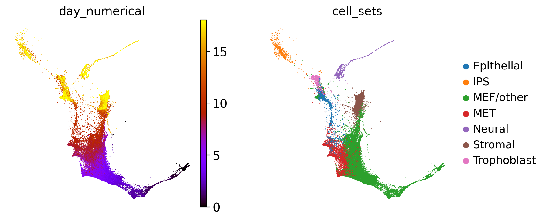
Each dot is a cell in the force-direction embedding, colored according to one of the 39 time-points of sequencing, from early (day 0, in black) to late (day 18, in yellow) (left) or coarse cell-set annotations (right). We created the cell_sets annotation by slightly modifying and combining the original annotations, introducing a MEF/other category that didn’t exist in the original data [Schiebinger et al., 2019].
Preprocess the data
This datset has already been normalized by total counts and log2-transformed. Further, highly variable genes have already been annotated. We can thus direclty compute a PCA representation and a k-NN graph, which we’ll need later on.
sc.pp.pca(adata)
sc.pp.neighbors(adata, random_state=0)
Reconstruct differentiation trajectories across time points
Run moscot to couple cells
With moscot, we couple cells across time points using optimal transport (OT), as pioneered by Waddington-OT [Schiebinger et al., 2019]. moscot scales to millions of cells and supports multi-modal data []. We demonstrate the most basic use-case here: linking a smaller-scale unimodal scRNA-seq dataset across experimental time points.
Note
moscot can do much more! To learn how to incorporate multimodal information, millions of cells, and additional spatial information, check out the documentation, including many tutorials. Additionally, to include lineage-traced data, check out the moscot-lineage (moslin) tutorial.
Importantly, everything we demonstrate here works exactly the same if you include these additional data modalities! The couplings just get better, and additional downstream analysis becomes available.
The first step is to set up a TemporalProblem. If you have additional spatial or lineage information, you can use the SpatioTemporalProblem or the LineageProblem, respectively.
tp = TemporalProblem(adata)
Next, we adjust the marginals for cellular growth- and death using score_genes_for_marginals().
tp = tp.score_genes_for_marginals(
    gene_set_proliferation="mouse", gene_set_apoptosis="mouse"
)
WARNING: genes are not in var_names and ignored: Index(['Mlf1ip'], dtype='object')
WARNING: genes are not in var_names and ignored: Index(['Ccnd2', 'Clca2'], dtype='object')
Visualize the computed proliferation and apoptosis scores in the embedding.
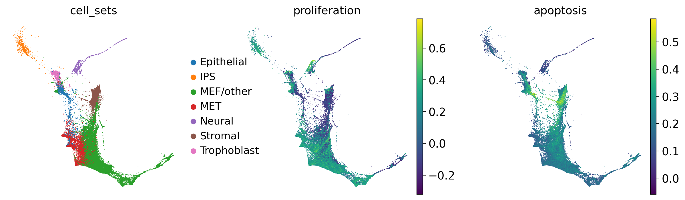
sc.pl.embedding(
    adata, basis="force_directed", color=["cell_sets", "proliferation", "apoptosis"]
)
Following the original Waddington OT publication, we use local PCAs, computed separately for each pair of time points, to calulate distances among cells [Schiebinger et al., 2019]. Accordingly, we prepare the TemporalProblem without passing a joint_attr, this automatically computes local PCAs.
tp = tp.prepare(time_key="day")
INFO     Computing pca with `n_comps=30` for `xy` using `adata.X`
INFO     Computing pca with `n_comps=30` for `xy` using `adata.X`
INFO     Computing pca with `n_comps=30` for `xy` using `adata.X`
INFO     Computing pca with `n_comps=30` for `xy` using `adata.X`
INFO     Computing pca with `n_comps=30` for `xy` using `adata.X`
INFO     Computing pca with `n_comps=30` for `xy` using `adata.X`
INFO     Computing pca with `n_comps=30` for `xy` using `adata.X`
INFO     Computing pca with `n_comps=30` for `xy` using `adata.X`
INFO     Computing pca with `n_comps=30` for `xy` using `adata.X`
INFO     Computing pca with `n_comps=30` for `xy` using `adata.X`
INFO     Computing pca with `n_comps=30` for `xy` using `adata.X`
INFO     Computing pca with `n_comps=30` for `xy` using `adata.X`
INFO     Computing pca with `n_comps=30` for `xy` using `adata.X`
INFO     Computing pca with `n_comps=30` for `xy` using `adata.X`
INFO     Computing pca with `n_comps=30` for `xy` using `adata.X`
INFO     Computing pca with `n_comps=30` for `xy` using `adata.X`
INFO     Computing pca with `n_comps=30` for `xy` using `adata.X`
INFO     Computing pca with `n_comps=30` for `xy` using `adata.X`
INFO     Computing pca with `n_comps=30` for `xy` using `adata.X`
INFO     Computing pca with `n_comps=30` for `xy` using `adata.X`
INFO     Computing pca with `n_comps=30` for `xy` using `adata.X`
INFO     Computing pca with `n_comps=30` for `xy` using `adata.X`
INFO     Computing pca with `n_comps=30` for `xy` using `adata.X`
INFO     Computing pca with `n_comps=30` for `xy` using `adata.X`
INFO     Computing pca with `n_comps=30` for `xy` using `adata.X`
INFO     Computing pca with `n_comps=30` for `xy` using `adata.X`
INFO     Computing pca with `n_comps=30` for `xy` using `adata.X`
INFO     Computing pca with `n_comps=30` for `xy` using `adata.X`
INFO     Computing pca with `n_comps=30` for `xy` using `adata.X`
INFO     Computing pca with `n_comps=30` for `xy` using `adata.X`
INFO     Computing pca with `n_comps=30` for `xy` using `adata.X`
INFO     Computing pca with `n_comps=30` for `xy` using `adata.X`
INFO     Computing pca with `n_comps=30` for `xy` using `adata.X`
INFO     Computing pca with `n_comps=30` for `xy` using `adata.X`
INFO     Computing pca with `n_comps=30` for `xy` using `adata.X`
INFO     Computing pca with `n_comps=30` for `xy` using `adata.X`
INFO     Computing pca with `n_comps=30` for `xy` using `adata.X`
INFO     Computing pca with `n_comps=30` for `xy` using `adata.X`
In the final step, we solve one OT problem per time point pair, probabilistically matching early to late cells [Peyré et al., 2019].
tp = tp.solve(epsilon=0.05, tau_a=0.95, scale_cost="mean")
INFO     Solving `38` problems
INFO     Solving problem BirthDeathProblem[stage='prepared', shape=(561, 489)].
INFO     Solving problem BirthDeathProblem[stage='prepared', shape=(1785, 1756)].
INFO     Solving problem BirthDeathProblem[stage='prepared', shape=(1620, 2118)].
INFO     Solving problem BirthDeathProblem[stage='prepared', shape=(755, 762)].
INFO     Solving problem BirthDeathProblem[stage='prepared', shape=(685, 954)].
INFO     Solving problem BirthDeathProblem[stage='prepared', shape=(1749, 1641)].
INFO     Solving problem BirthDeathProblem[stage='prepared', shape=(866, 881)].
INFO     Solving problem BirthDeathProblem[stage='prepared', shape=(919, 755)].
INFO     Solving problem BirthDeathProblem[stage='prepared', shape=(477, 1749)].
INFO     Solving problem BirthDeathProblem[stage='prepared', shape=(495, 579)].
INFO     Solving problem BirthDeathProblem[stage='prepared', shape=(579, 525)].
INFO     Solving problem BirthDeathProblem[stage='prepared', shape=(1656, 1284)].
INFO     Solving problem BirthDeathProblem[stage='prepared', shape=(869, 1151)].
INFO     Solving problem BirthDeathProblem[stage='prepared', shape=(775, 1656)].
INFO     Solving problem BirthDeathProblem[stage='prepared', shape=(1189, 869)].
INFO     Solving problem BirthDeathProblem[stage='prepared', shape=(1725, 1818)].
INFO     Solving problem BirthDeathProblem[stage='prepared', shape=(602, 579)].
INFO     Solving problem BirthDeathProblem[stage='prepared', shape=(958, 952)].
INFO     Solving problem BirthDeathProblem[stage='prepared', shape=(917, 1047)].
INFO     Solving problem BirthDeathProblem[stage='prepared', shape=(1641, 1725)].
INFO     Solving problem BirthDeathProblem[stage='prepared', shape=(525, 602)].
INFO     Solving problem BirthDeathProblem[stage='prepared', shape=(527, 514)].
INFO     Solving problem BirthDeathProblem[stage='prepared', shape=(1284, 958)].
INFO     Solving problem BirthDeathProblem[stage='prepared', shape=(1151, 917)].
INFO     Solving problem BirthDeathProblem[stage='prepared', shape=(1818, 2241)].
INFO     Solving problem BirthDeathProblem[stage='prepared', shape=(2241, 1785)].
INFO     Solving problem BirthDeathProblem[stage='prepared', shape=(1756, 1620)].
INFO     Solving problem BirthDeathProblem[stage='prepared', shape=(919, 685)].
INFO     Solving problem BirthDeathProblem[stage='prepared', shape=(952, 919)].
INFO     Solving problem BirthDeathProblem[stage='prepared', shape=(579, 527)].
INFO     Solving problem BirthDeathProblem[stage='prepared', shape=(1134, 866)].
INFO     Solving problem BirthDeathProblem[stage='prepared', shape=(762, 561)].
INFO     Solving problem BirthDeathProblem[stage='prepared', shape=(514, 919)].
INFO     Solving problem BirthDeathProblem[stage='prepared', shape=(881, 477)].
INFO     Solving problem BirthDeathProblem[stage='prepared', shape=(1047, 999)].
INFO     Solving problem BirthDeathProblem[stage='prepared', shape=(489, 495)].
INFO     Solving problem BirthDeathProblem[stage='prepared', shape=(2118, 775)].
INFO     Solving problem BirthDeathProblem[stage='prepared', shape=(954, 1189)].
Above, epsilon and tau_a control the amount of entropic regularization and unbalancedness on the source marginal, respectively. Higher entropic regularization speeds up the optimization and improves statistical properties of the solution [Cuturi, 2013]; unbalancedness makes the solution more robust with respect to uncertain cellular growth rates and biased cell sampling [Chizat et al., 2018, Schiebinger et al., 2019].
Set up the RealTimeKernel
The RealTimeKernel is CellRank’s interface with time-course data; it can load cellular couplings computed with moscot or Waddington OT.
tmk = RealTimeKernel.from_moscot(tp)
To get from a set of OT transport maps to a Markov chain describing a biological system, we do the following:
we sparsify OT transport maps by removing entries below a certain threshold; entropic regularization yields dense matrices which would make CellRank analysis very slow.
we use OT transport maps and molecular similarity to model transitions across and within time points, respectively.
we row-normalize the resulting cell-cell transition matrix (including all time points) and construct the Markov chain.
tmk.compute_transition_matrix(self_transitions="all", conn_weight=0.2, threshold="auto")
Visualize the recovered dynamics
We can visualize the cellular dynamics described by this Markov chain by sampling random walks.
tmk.plot_random_walks(
    max_iter=500,
    start_ixs={"day": 0.0},
    basis="force_directed",
    seed=0,
    dpi=150,
    size=30,
)
Black and yellow dots denote random walks starting and finishing points, respectively. Random walks mostly finish in the iPSC, Neural, Stromal, Trophoblast and Epithelial cell sets.
Another way to visualize the reconstructed dynamics is by plotting the probability mass flow in time [Mittnenzweig et al., 2021].
ax = tmk.plot_single_flow(
    cluster_key="cell_sets",
    time_key="day",
    cluster="MEF/other",
    min_flow=0.1,
    xticks_step_size=4,
    show=False,
    clusters=["MEF/other", "MET", "Stromal"],
)

_ = ax.set_xticklabels(ax.get_xticklabels(), rotation=90)
Closing matters
What’s next?
In this tutorial, you learned how CellRank can be used to compute a transition matrix based on experimental time points and how the transition matrix can be visualized in low dimensions. The real power of CellRank comes in when you use estimators to analyze the transition matrix directly in high dimensions. For the next steps, we recommend to:
go through the initial and terminal states tutorial to learn how to use the transition matrix to automatically identify initial and terminal states.
take a look at the
APIto learn about parameters you can use to adapt these computations to your data, and trying this out on your own data.read the Waddington-OT paper or the
moscotpreprint to learn more about linking cells across time points [Schiebinger et al., 2019].
Package versions
session_info2.session_info()