Getting Started with CellRank

Preliminaries

CellRank is a software toolkit to study dynamical biological processes, like development, regeneration, cancer or reprogramming, based on multi-view single-cell genomics data [Lange et al., 2022], including RNA velocity [Bergen et al., 2020, La Manno et al., 2018], developmental potentials [Gulati et al., 2020], pseudotemporal orderings [Bendall et al., 2014, Haghverdi et al., 2016, Setty et al., 2019, Trapnell et al., 2014], (spatial) time course studies [Schiebinger et al., 2019], lineage-traced data [Alemany et al., 2018, Forrow and Schiebinger, 2021, Raj et al., 2018, Spanjaard et al., 2018], metabolic labels [Battich et al., 2020, Erhard et al., 2019, Qiu et al., 2020, Qiu et al., 2022], and more.

Oftentimes, the type of downstream analysis does not depend on the modality that was used to estimate cellular transitions - that’s why we modularized CellRank into kernels, which compute cell-cell transition matrices, and estimators, which analyze the transition matrices.

In this tutorial, you will learn how to:

• use CellRank kernels to compute a transition matrix of cellular dynamics.

• use CellRank estimators to analyze the transition matrix, including the computation of fate probabilities, driver genes, and gene expression trends.

• read and write CellRank kernels.

This tutorial notebook can be downloaded using the following link.

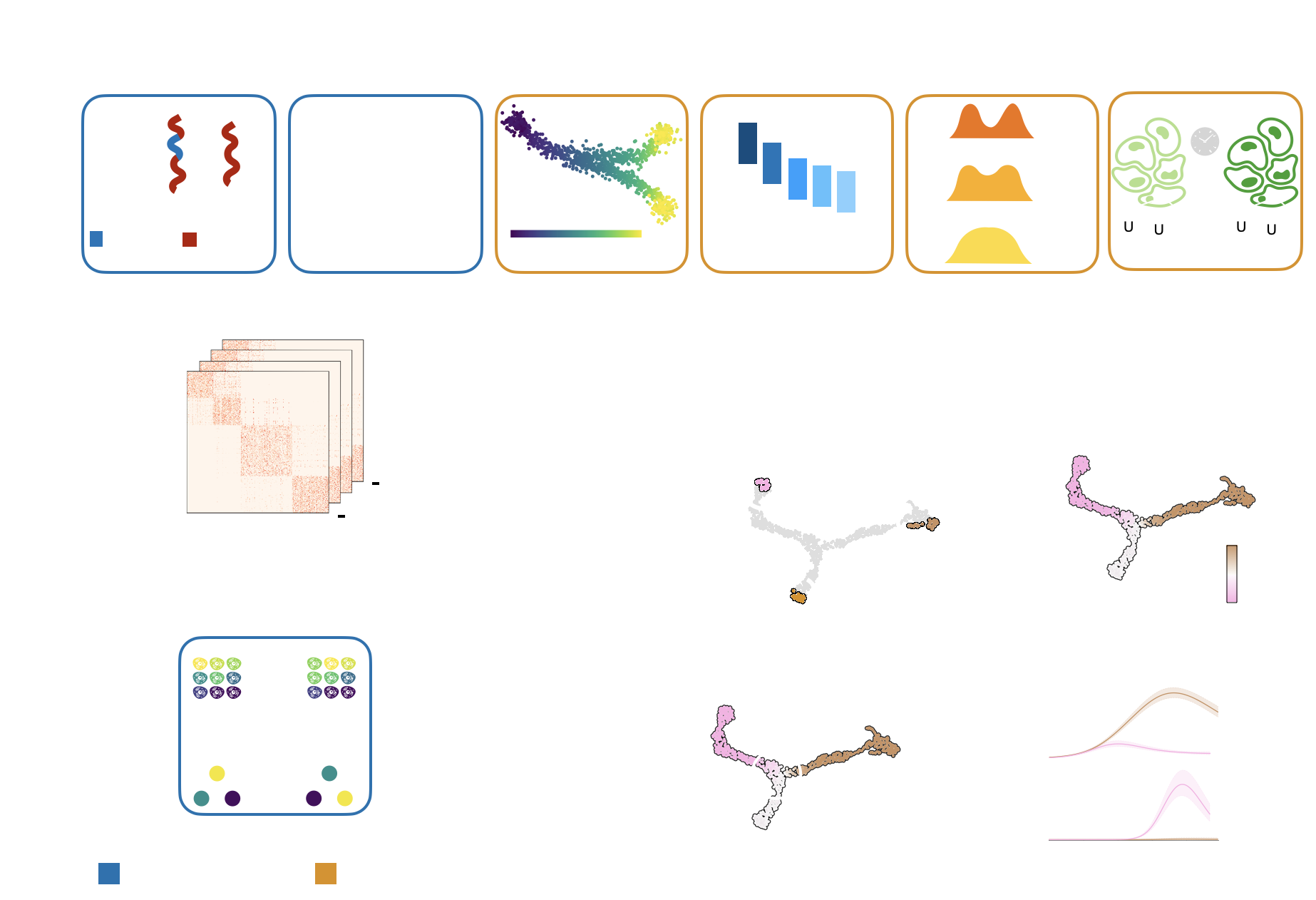
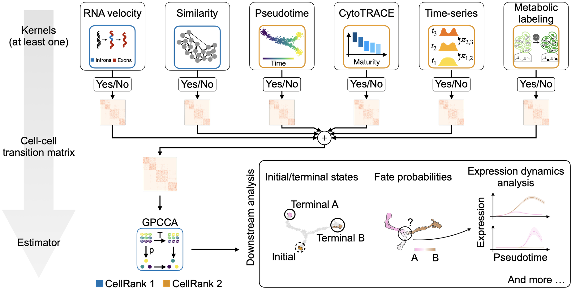
A unified fate-mapping framework: CellRank is composed of kernels, which compute a cell-cell transition matrix, and estimators, which analyze transition matrices to reveal initial & terminal states, fate probabilities, driver genes, and more.

Note

If you want to run this on your own data, you will need:

• a scRNA-seq dataset for which you can compute a cell-cell transition matrix using any CellRank kernel.

Note

If you encounter any bugs in the code, our if you have suggestions for new features, please open an issue. If you have a general question or something you would like to discuss with us, please post on the scverse discourse.

Import packages & data

%load_ext autoreload
%autoreload 2

import sys

if "google.colab" in sys.modules:
    !pip install -q git+https://github.com/scverse/cellrank

import cellrank as cr
import scanpy as sc
import session_info2

sc.set_figure_params(frameon=False, dpi=100)
cr.settings.logging_level = "INFO"

import warnings

warnings.simplefilter("ignore", category=UserWarning)

To demonstrate the appproach in this tutorial, we will use a scRNA-seq dataset of human bone marrow, which can be conveniently acessed through bone_marrow [Setty et al., 2019].

adata = cr.datasets.bone_marrow()
adata

AnnData object with n_obs × n_vars = 5780 × 27876
    obs: 'clusters', 'palantir_pseudotime', 'palantir_diff_potential'
    var: 'palantir'
    uns: 'clusters_colors', 'palantir_branch_probs_cell_types'
    obsm: 'MAGIC_imputed_data', 'X_tsne', 'palantir_branch_probs'
    layers: 'spliced', 'unspliced'

Preprocess the data

Filter and normalize.

sc.pp.filter_genes(adata, min_cells=5)
sc.pp.normalize_total(adata, target_sum=1e4)

sc.pp.log1p(adata)
sc.pp.highly_variable_genes(adata, n_top_genes=3000)

Compute PCA and k-nearest neighbor (k-NN) graph.

sc.tl.pca(adata, random_state=0)
sc.pp.neighbors(adata, random_state=0)

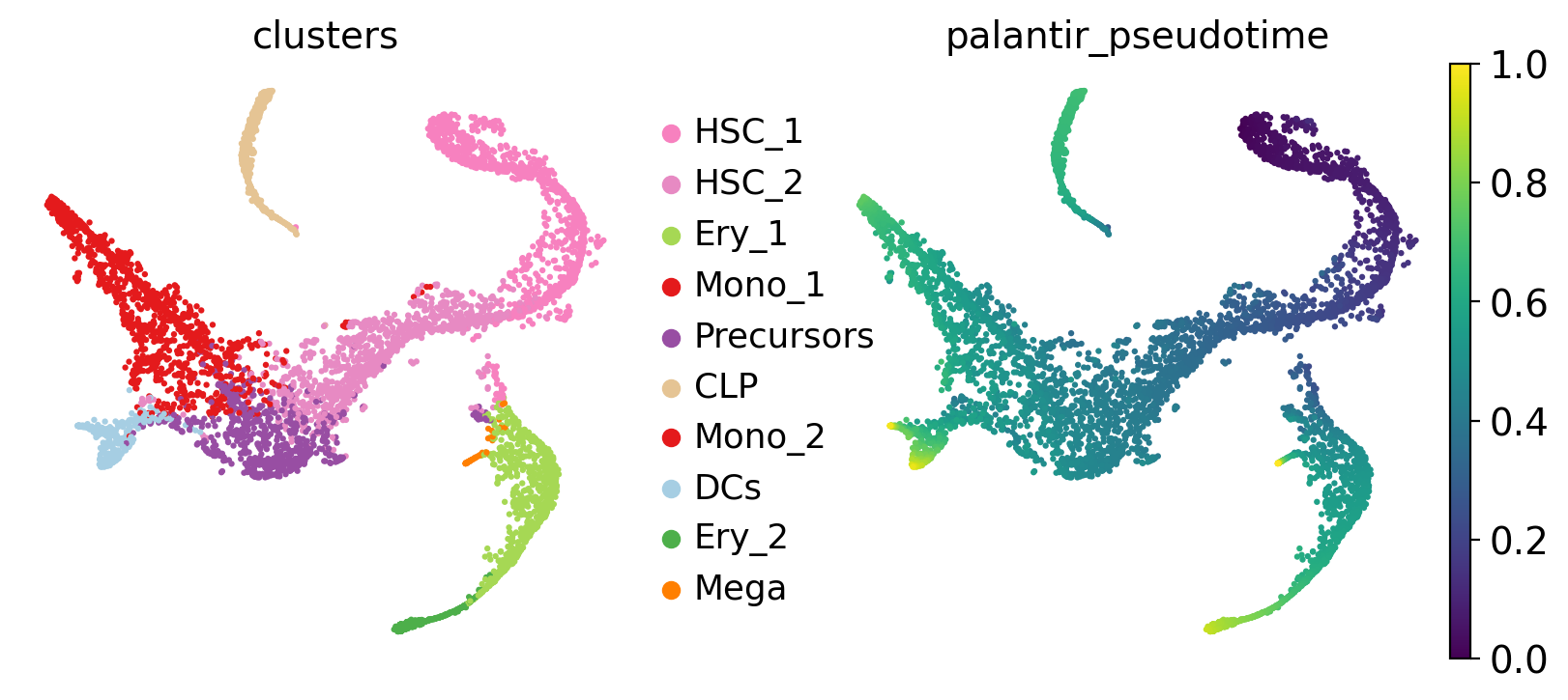
Visualize this data, using the t-SNE embedding, cluster labels and Palantir pseudotime provided with the original study [Setty et al., 2019].

sc.pl.embedding(adata, basis="tsne", color=["clusters", "palantir_pseudotime"])

Working with kernels

Set up a kernel

To construct a transition matrix, CellRank offers a number of kernel classes in kernels. To demonstrate the concept, we’ll use the PseudotimeKernel which biases k-NN graph edges to point into the direction of increasing pseudotime, inspired by Palantir [Setty et al., 2019].

For a full list of kernels, check out our API. To initialize a kernel object, simply run the following:

from cellrank.kernels import PseudotimeKernel

pk = PseudotimeKernel(adata, time_key="palantir_pseudotime")

Note that kernels need an anndata.AnnData object to read data from it - CellRank is part of the Scanpy/AnnData ecosystem. The only exception to this is the cellrank.kernels.PrecomputedKernel which directly accepts a transition matrix, thus making it possible to interface to CellRank from outside the scanpy/AnnData world.

To learn more about our kernel object, we can print it.

pk

PseudotimeKernel[n=5780]

There isn’t very much here yet! Let’s use this kernel to compute a cell-cell transition_matrix.

pk.compute_transition_matrix()

INFO     Computing transition matrix based on pseudotime                                                           

INFO         Finish (0.87s)                                                                                        

PseudotimeKernel[n=5780, dnorm=False, scheme='hard', frac_to_keep=0.3]

If we print the kernel again, we can inspect the parameters that were used to compute this transition matrix.

pk

PseudotimeKernel[n=5780, dnorm=False, scheme='hard', frac_to_keep=0.3]

To get a first impression of the cellular dynamics in this dataset, we can simulate random walks on the Markov chain implied by the transition matrix, starting from hematopoietic stem cells (HSCs), and visualize these in the t-SNE embedding.

pk.plot_random_walks(
    seed=0,
    n_sims=100,
    start_ixs={"clusters": "HSC_1"},
    basis="tsne",
    max_iter=100,
    legend_loc="on data",
    color="clusters",
)

INFO     Simulating 100 random walks of maximum length 100                                                         

INFO         Finish (1.22s)                                                                                        
INFO     Plotting random walks                                                                                     

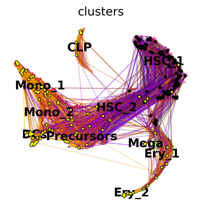
Black and yellow dots indicate random walk start and terminal cells, respectively. Overall, this reflects the known differentiation hierachy in human hematopoiesis.

See also

To learn more about the PseudotimeKernel, see CellRank Meets Pseudotime.

Kernel overview

There exist CellRank kernels for many different data modalities. Each modality and biological system comes with its own strenghts and limitations, so it’s important to choose the kernel carefully. We provide some guidance in the figure below. However, please check the kernel API for a complete and up-to-date list, as new kernels will come.

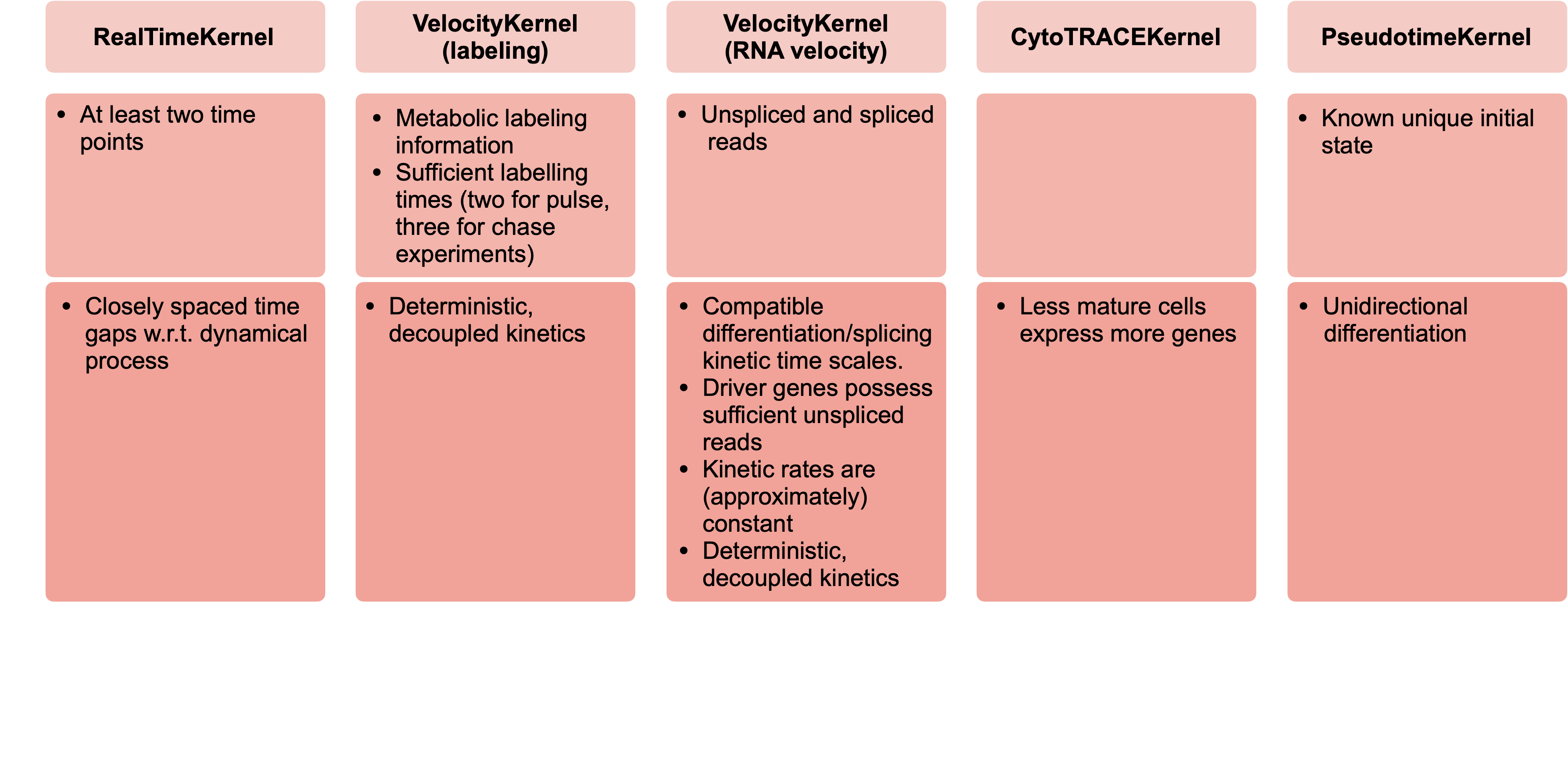
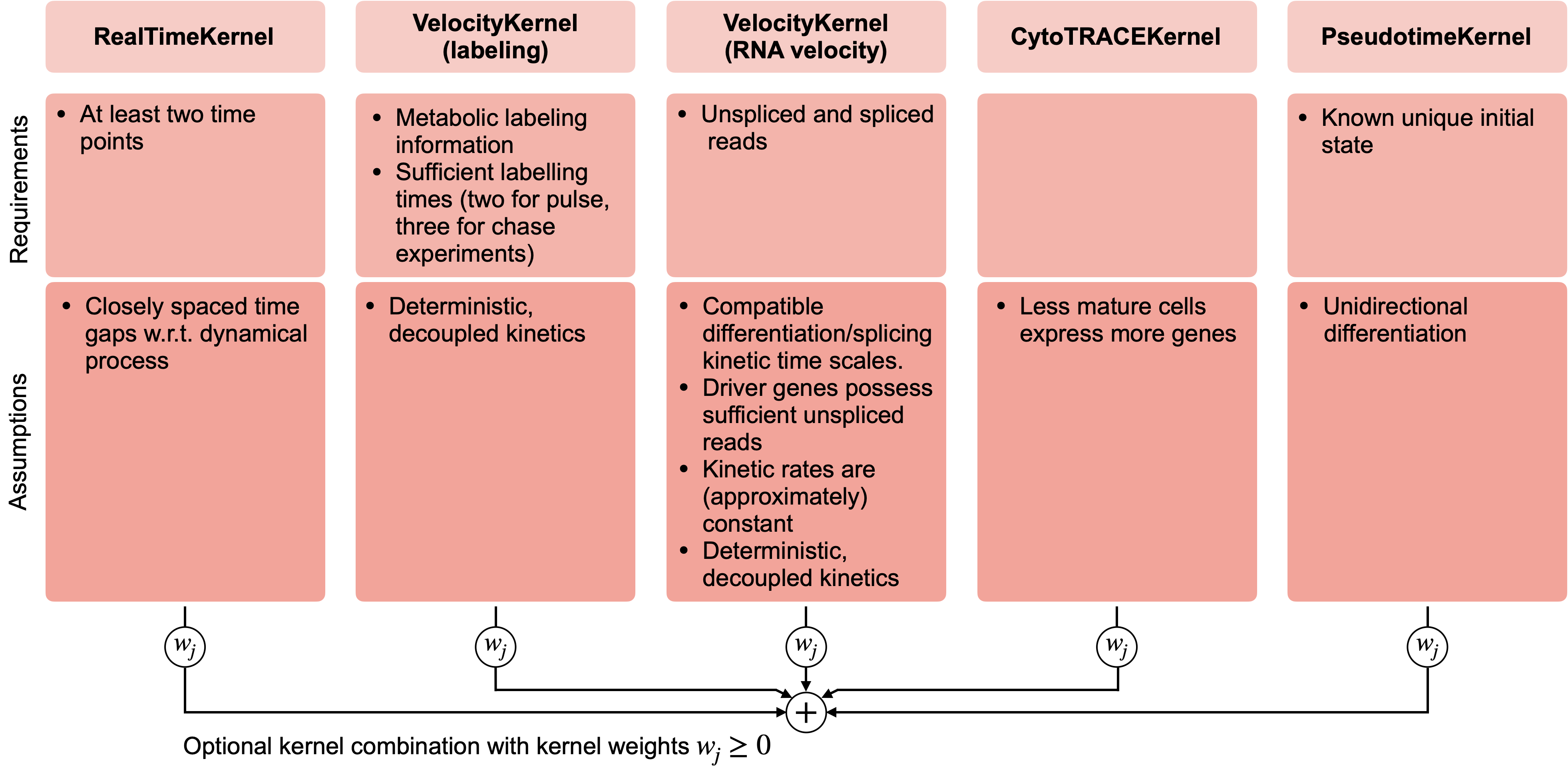
A guide to kernel choice: CellRank kernels support different data modalities and biological systems. Each comes with its own assumptions and limitations.

If you already have a cell-cell transition matrix for your data, you can pass that directly using the cellrank.kernels.PrecomputedKernel, CellRank’s interface with external methods.

Combining different kernels

Any two kernels can be globally combined via a weighted mean. To demonstrate this, let’s set up an additional cellrank.kernels.ConnectivityKernel, based on gene expression similarity.

from cellrank.kernels import ConnectivityKernel

ck = ConnectivityKernel(adata).compute_transition_matrix()

INFO     Computing transition matrix based on adata.obsp['connectivities']                                         
INFO         Finish (0.01s)                                                                                        

Print the kernel to see some properties

ck

ConnectivityKernel[n=5780, dnorm=True, key='connectivities']

Combine with the PseudotimeKernel PseudotimeKernel from above.

combined_kernel = 0.8 * pk + 0.2 * ck
combined_kernel

(0.8 * PseudotimeKernel[n=5780, dnorm=False, scheme='hard', frac_to_keep=0.3] + 0.2 * ConnectivityKernel[n=5780, dnorm=True, key='connectivities'])

This works for any combination of kernels, and generalizes to more than two kernels. Kernel combinations allow you to use distinct sources of information to describe cellular dynamics.

Writing and reading a kernel

Sometimes, we might want to write the kernel to disk, to either continue with the analysis later on, or to pass it to someone else. This can be easily done; simply write the kernel to adata, and write adata to file:

pk.write_to_adata()
adata.write("hematopoiesis.h5ad")

To continue with the analysis, we read the anndata.AnnData object from disk, and initialize a new kernel from the AnnData object.

adata = sc.read("hematopoiesis.h5ad")
pk_new = cr.kernels.PseudotimeKernel.from_adata(adata, key="T_fwd")
pk_new

PseudotimeKernel[n=5780, dnorm=False, frac_to_keep=0.3, scheme='hard']

Working with estimators

Set up an estimator

Estimators take a kernel object and offer methods to analyze it. The main objective is to decompose the state space into a set of macrostates that represent the slow-time scale dynamics of the process. A subset of these macrostates will be the initial or terminal states of the process, the remaining states will be intermediate transient states. CellRank currently offers two estimator classes in cellrank.estimators:

• CFLARE: Clustering and Filtering Left And Right Eigenvectors. Heuristic method based on the spectrum of the transition matrix.

• GPCCA: Generalized Perron Cluster Cluster Analysis: project the Markov chain onto a small set of macrostates using a Galerkin projection which maximizes the self-transition probability for the macrostates, [Reuter et al., 2019, Reuter et al., 2018].

We recommend the CFLARE estimator; let’s start by initializing it.

from cellrank.estimators import GPCCA

g = GPCCA(pk_new)
print(g)

GPCCA[kernel=PseudotimeKernel[n=5780], initial_states=None, terminal_states=None]

Identify initial & terminal states

Fit the estimator to compute macrostates of cellular dynamics; these may include initial, terminal and intermediate states.

Let’s start by computing a Schur decomposition of the data.

g.compute_schur()
g.plot_spectrum(real_only=True)

INFO     Computing Schur decomposition                                                                             
INFO     When computing macrostates, choose a number of states NOT in ``                                           
INFO     Adding `adata.uns['eigendecomposition_fwd']`                                                              
                `.schur_vectors`                                                                                   
                `.schur_matrix`                                                                                    
                `.eigendecomposition`                                                                              
             Finish (1.90s)                                                                                        

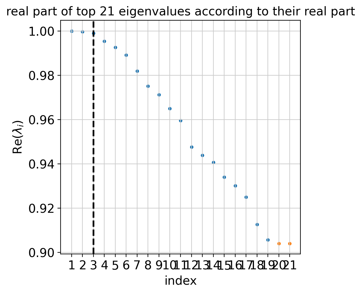
The plot above shows real and complex conjugate eigenvalue pairs and makes a suggestion for how many macrostates to compute. Next, we compute and visualize macrostates.

g.compute_macrostates(n_states=10, cluster_key="clusters")
g.plot_macrostates(which="all", basis="tsne")

INFO     Computing 10 macrostates                                                                                  
WARNING  Color sequence contains non-unique elements                                                               
INFO     Adding `.macrostates`                                                                                     
                `.macrostates_memberships`                                                                         
                `.coarse_T`                                                                                        
                `.coarse_initial_distribution                                                                      
                `.coarse_stationary_distribution`                                                                  
                `.schur_vectors`                                                                                   
                `.schur_matrix`                                                                                    
                `.eigendecomposition`                                                                              
             Finish (4.01s)                                                                                        

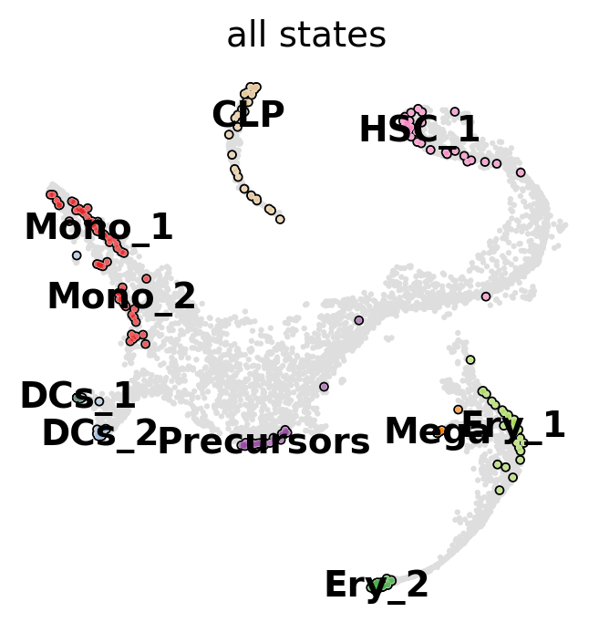
For each macrostate, the algorithm computes an associated stability value. Let’s use the most stable macrostates as terminal states [Lange et al., 2022, Reuter et al., 2019, Reuter et al., 2018].

g.predict_terminal_states(method="top_n", n_states=6)
g.plot_macrostates(which="terminal", basis="tsne")

INFO     Adding `adata.obs['term_states_fwd']`                                                                     
                `adata.obs['term_states_fwd_probs']`                                                               
                `.terminal_states`                                                                                 
                `.terminal_states_probabilities`                                                                   
                `.terminal_states_memberships                                                                      
             Finish`                                                                                               

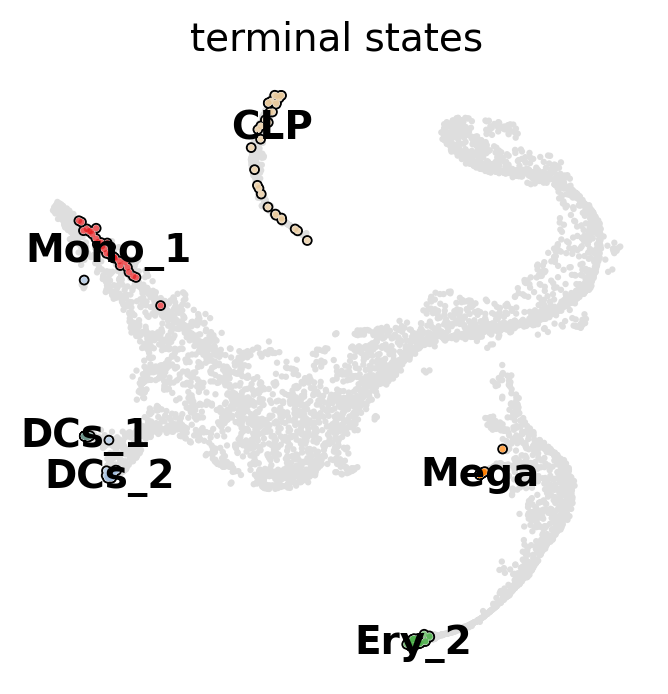
This correctly identified all major terminal states in this dataset. CellRank can also identify initial states - in this dataset, that does not make too much sense though, as the initial state was manually passed to Palantir to root the pseudotime computation.

See also

To learn more about initial and terminal state identification, see Computing Initial and Terminal States.

Compute fate probabilities and driver genes

We can now compute how likely each cell is to reach each terminal state using compute_fate_probabilities().

g.compute_fate_probabilities()
g.plot_fate_probabilities(legend_loc="right", basis="tsne")

INFO     Computing fate probabilities                                                                              

INFO     Adding `adata.obsm['lineages_fwd']`                                                                       
                `.fate_probabilities`                                                                              
             Finish (0.23s)                                                                                        

[0]PETSC ERROR: ------------------------------------------------------------------------
[0]PETSC ERROR: Caught signal number 13 Broken Pipe: Likely while reading or writing to a socket
[0]PETSC ERROR: Try option -start_in_debugger or -on_error_attach_debugger
[0]PETSC ERROR: or see https://petsc.org/release/faq/#valgrind and https://petsc.org/release/faq/
[0]PETSC ERROR: configure using --with-debugging=yes, recompile, link, and run 
[0]PETSC ERROR: to get more information on the crash.

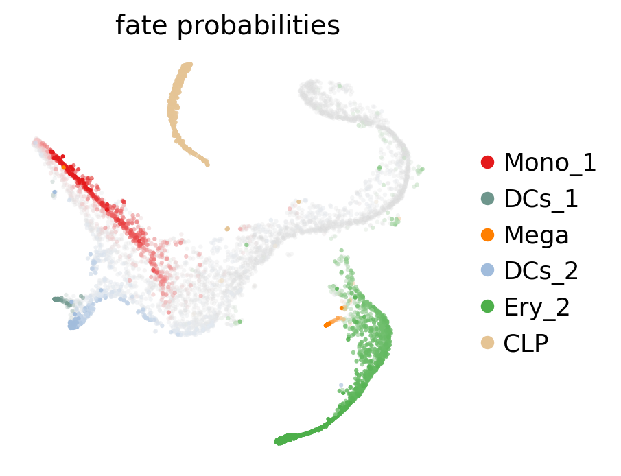
The plot above combines fate probabilities towards all terminal states, each cell is colored according to its most likely fate; color intensity reflects the degree of lineage priming. We could equally plot fate probabilities separately for each terminal state, or we can visualize them jointly in a circular projection [Lange et al., 2022, Velten et al., 2017].

cr.pl.circular_projection(adata, keys="clusters", legend_loc="right")

INFO     Solving TSP for `6` states                                                                                

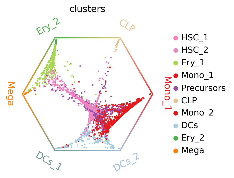
Each dot represents a cell, colored by cluster labels. Cells are arranged inside the circle according to their fate probabilities; fate biased cells are placed next to their corresponding corner while naive cells are placed in the middle.

To infer putative driver genes for any of these trajectories, we correlate expression values with fate probabilities.

mono_drivers = g.compute_lineage_drivers(lineages="Mono_1")
mono_drivers.head(10)

INFO     Adding `adata.varm['terminal_lineage_drivers']`                                                           
                `.lineage_drivers`                                                                                 
             Finish (0.65s)                                                                                        

	Mono_1_corr	Mono_1_pval	Mono_1_qval	Mono_1_ci_low	Mono_1_ci_high
index
AZU1	0.740418	0.0	0.0	0.728544	0.751847
MPO	0.735347	0.0	0.0	0.723278	0.746967
ELANE	0.715912	0.0	0.0	0.703108	0.728252
CTSG	0.700536	0.0	0.0	0.687165	0.713432
PRTN3	0.649584	0.0	0.0	0.634428	0.664241
RNASE2	0.582030	0.0	0.0	0.564722	0.598825
SRGN	0.567426	0.0	0.0	0.549686	0.584654
RPS19	0.559501	0.0	0.0	0.541531	0.576960
CFD	0.538689	0.0	0.0	0.520131	0.556738
RAB32	0.537442	0.0	0.0	0.518850	0.555526

See also

To learn more about fate probabilities and driver genes, see Estimating Fate Probabilities and Driver Genes.

Visualize expression trends

Given fate probabilities and a pseudotime, we can plot trajectory-specific gene expression trends. Specifically, we fit Generalized Additive Models (GAMs), weighthing each cells contribution to each trajectory according to its vector of fate probabilities. We start by initializing a model.

model = cr.models.GAM(adata)

Note

The GAMR uses the R package mgcv for parameter fitting; this requires you to have rpy2 installed. To avoid this and remain entirely in python, you can use cellrank.models.GAM, which uses pyGAM for parameter fitting.

With the model initialized, we can visualize gene dynamics along specific trajectories.

with warnings.catch_warnings():
    warnings.simplefilter("ignore")

    cr.pl.gene_trends(
        adata,
        model=model,
        genes=["GATA1", "CD34", "IRF8", "MPO"],
        same_plot=True,
        ncols=2,
        time_key="palantir_pseudotime",
        hide_cells=True,
    )

INFO     Computing trends using 1 core(s)                                                                          

INFO         Finish (1.20s)                                                                                        
INFO     Plotting trends                                                                                           

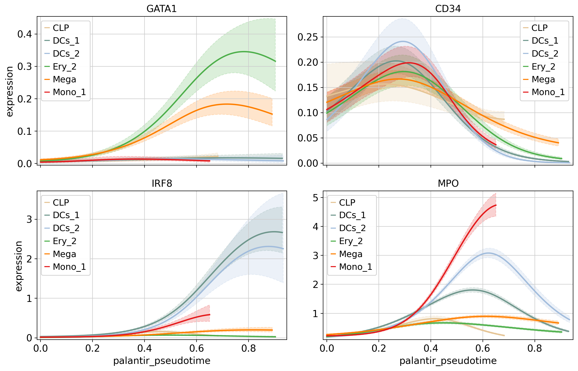
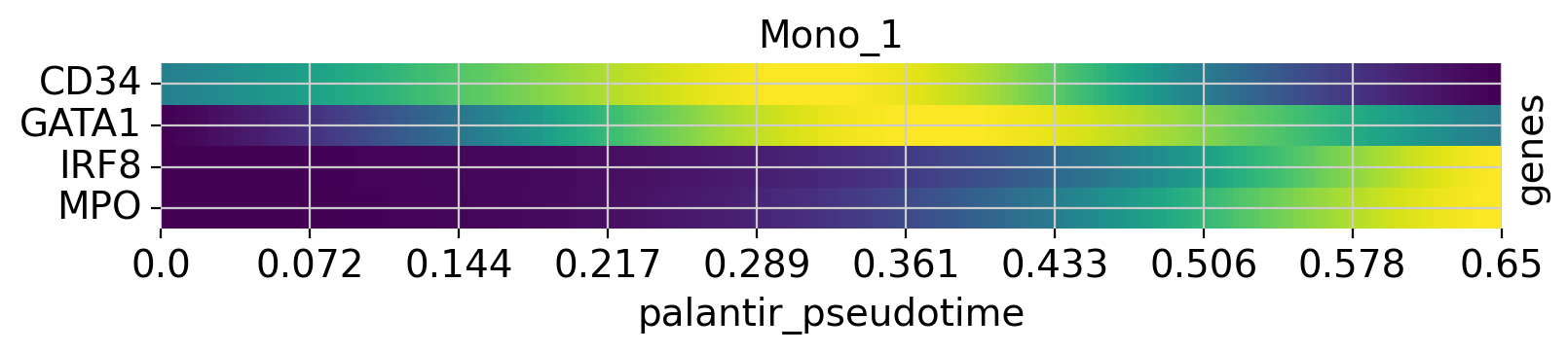
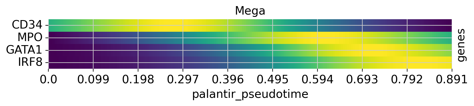
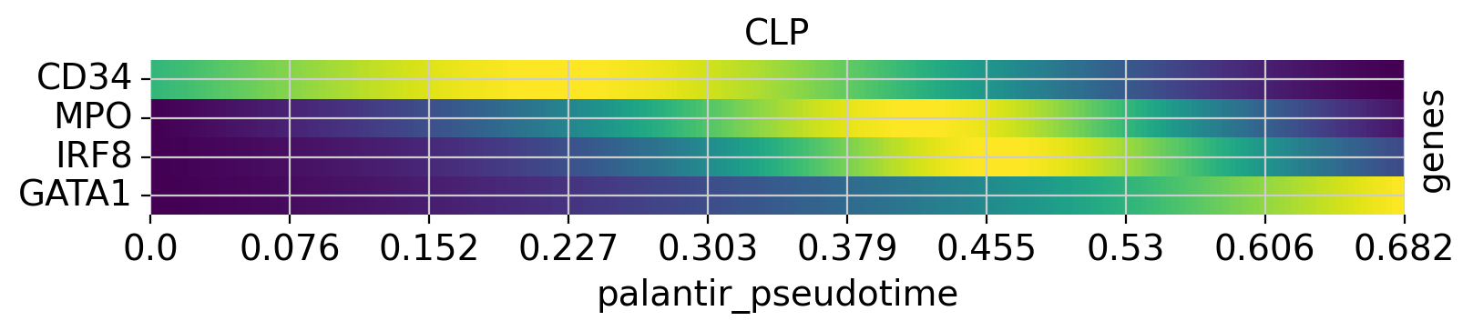
Above, we grouped expression trends by gene, and visualized several trajectories per panel. We can also do it the other way round - group expression trends by trajectory, visualize several genes per panel. While this is possible using the line plots from above (set transpose=True), we’ll demonstrate it using heatmaps.

with warnings.catch_warnings():
    warnings.simplefilter("ignore")

    cr.pl.heatmap(
        adata,
        model=model,
        genes=["GATA1", "CD34", "IRF8", "MPO"],
        lineages=["Mono_1", "Mega", "CLP"],
        time_key="palantir_pseudotime",
        cbar=False,
        show_all_genes=True,
    )

INFO     Computing trends using 1 core(s)                                                                          

INFO         Finish (0.63s)                                                                                        

See also

To learn more about gene trend visualization and clustering, see Visualizing and Clustering Gene Expression Trends.

Closing matters

Creating a new kernel - contributing to CellRank

If you have you own method in mind for computing a cell-cell transition matrix, potentially based on some new data modality, consider including it as a kernel in CellRank. That way, you benefit from CellRank’s established interfaces with packages like scanpy or AnnData, can take advantage of existing downstream analysis capabilities, and immediately reach a large audience of existing CellRank users.

See also

To learn more about creating your own kernel, see TODO.

What’s next?

In this tutorial, you learned the basics of CellRank. For the next steps, we recommend to:

• explore the various CellRank kernels (REF) and corresponding tutorials.

• take a look at the API to learn about parameter values you can use to adapt these computations to your data.

• dive deeper into initial and terminal states, fate probabilities, and gene expression trends.

Package versions

session_info2.session_info()