CellRank Meets CytoTRACE

Preliminaries

In this tutorial, you will learn how to:

• compute a developmental potential using our adapted CytoTRACE implementation [Gulati et al., 2020].

• set up CellRank’s CytoTRACEKernel to compute a transition matrix based on the CytoTRACE score.

• visualize the transition matrix in a low-dimensional embedding.

This tutorial notebook can be downloaded using the following link.

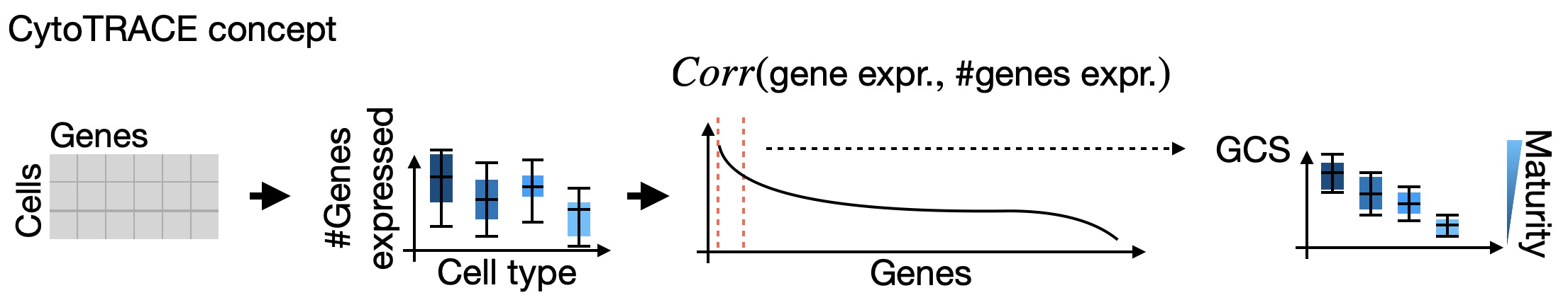
CytoTRACE estimates differentiation potential: Following the original CytoTRACE suggestion, we use the number of genes expressed per cell as a raw signal of differentiation status and apply several post-processing steps to increase robustness. The basic assumption behind this method is that naive cells on average express more genes compared to mature cells because they regulate their chromatin less tightly; we’ve observed this to work well for many early developmental datasets.

Note

A bottleneck in the original implementation was scalabilty of the post-processing steps [Gulati et al., 2020]; we therefore adapted the original CytoTRACE implementation to be much faster and memory efficient. We confirmed across several examples that our reimplementation yields biologically equivalent results (CITE). To get from the CytoTRACE pseudotime to a directed transition matrix, we use the general mechanism described in the pseudotime tutorial.

Note

If you want to run this on your own data, you will need:

• a scRNA-seq dataset which satisfies the CytoTRACE assumptions, i.e., naive cell states should on avarage express more genes. This is often the case for early develpmental stages.

Note

If you encounter any bugs in the code, our if you have suggestions for new features, please open an issue. If you have a general question or something you would like to discuss with us, please post on the scverse discourse.

Import packages & data

%load_ext autoreload
%autoreload 2

import sys

if "google.colab" in sys.modules:
    !pip install -q git+https://github.com/scverse/cellrank

import cellrank as cr
import scanpy as sc
import session_info2
from cellmapper import CellMapper

cr.settings.logging_level = "INFO"
sc.set_figure_params(frameon=False, dpi=100)

import warnings

warnings.simplefilter("ignore", category=UserWarning)

To demonstrate the appproach in this tutorial, we will use a scRNA-seq dataset of zebrafish embryogenesis assayed using drop-seq, restricted to the axial mesoderm lineage [Farrell et al., 2018]. This dataset can be acessed conveniently using zebrafish.

adata = cr.datasets.zebrafish()
adata

AnnData object with n_obs × n_vars = 2434 × 23974
    obs: 'Stage', 'gt_terminal_states', 'lineages'
    uns: 'Stage_colors', 'gt_terminal_states_colors', 'lineages_colors'
    obsm: 'X_force_directed'

Explore the data

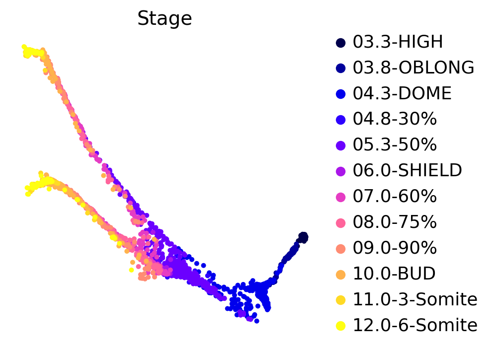
This zebrafish dataset contains 12 time-points spanning 3.3 - 12 hours past fertilization. We can use the original force-directed layout to plot cells, colored by developmental stage:

sc.pl.embedding(adata, basis="force_directed", color="Stage")

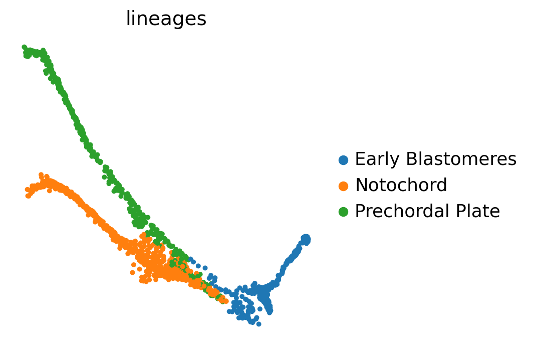
We can further look into the lineage assignments, computed in the original study using URD [Farrell et al., 2018]:

sc.pl.embedding(adata, basis="force_directed", color="lineages")

Preprocess

Before we can start applying the CytoTRACE kernel, we’ll have to do some basic preprocessing of the data.

# filter, normalize total counts and log-transform
sc.pp.filter_genes(adata, min_cells=10)
sc.pp.normalize_per_cell(adata)
sc.pp.log1p(adata)

# hvg annotation
sc.pp.highly_variable_genes(adata)
print(f"This detected {adata.var['highly_variable'].sum()} highly variable genes. ")

sc.tl.pca(adata)
sc.pp.neighbors(adata)

/scratch/tmp.59314195.mlange/ipykernel_566744/517370911.py:3: FutureWarning: Use `sc.pp.normalize_total` instead.
  sc.pp.normalize_per_cell(adata)

This detected 2392 highly variable genes. 

CytoTRACE uses imputed gene expression to calculate the differentiation potential score. We’ll simply use CellMapper for the imputation.

adata.layers["imputed"] = (
    CellMapper(adata).map(layer_key="X", use_rep="X_pca").query_imputed.X.copy()
)

INFO     Initialized CellMapper for self-mapping with 2434 cells.                                                  
INFO     Self-mapping mode detected. Computing only yx neighbors for efficiency (all neighbor matrices will contain
         the same information).                                                                                    
INFO     Using sklearn to compute 30 neighbors.                                                                    
INFO     Computing mapping matrix using kernel method 'umap'.                                                      
INFO     Mapping layer for key 'X' using direct multiplication                                                     
INFO     Imputed expression matrix with shape (2434, 13690) converted to AnnData object.                           
         Observation metadata from query and feature metadata from reference were linked (not copied).             
INFO     Expression for layer 'X' mapped and stored in query_imputed.X.                                            

Use developmental potential to direct differentiation

Compute the CytoTRACE score

Import the CytoTRACEKernel, initialize it using the preprocessed AnnData object and compute the CytoTRACE score:

from cellrank.kernels import CytoTRACEKernel

ctk = CytoTRACEKernel(adata).compute_cytotrace(layer="imputed")

INFO     Computing CytoTRACE score with `13690` genes                                                              
INFO     Adding `adata.obs['ct_score']`                                                                            
                `adata.obs['ct_pseudotime']`                                                                       
                `adata.obs['ct_num_exp_genes']`                                                                    
                `adata.var['ct_gene_corr']`                                                                        
                `adata.var['ct_correlates']`                                                                       
                `adata.uns['ct_params']`                                                                           
             Finish (0.14s)                                                                                        

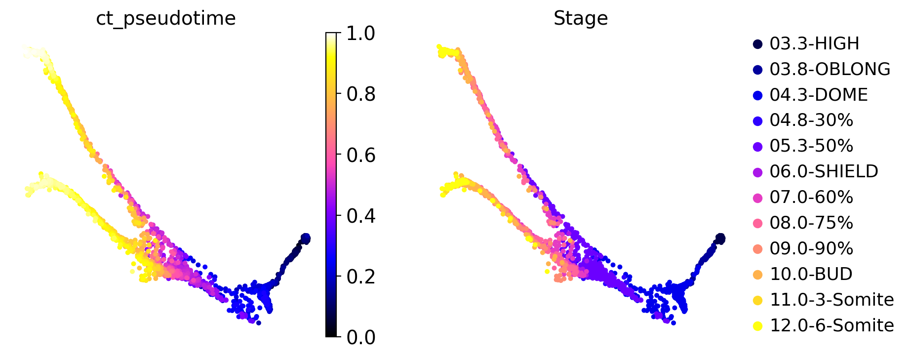
We can visually check that our computed CytoTRACE pseudotime correlates well with ground-truth real-time annotations:

sc.pl.embedding(
    adata,
    color=["ct_pseudotime", "Stage"],
    basis="force_directed",
    color_map="gnuplot2",
)

To make this a bit more quantitative, we can look at the distribution of our CytoTRACE pseudotime over real time points and show this via violin plots:

sc.pl.violin(adata, keys=["ct_pseudotime"], groupby="Stage", rotation=90)

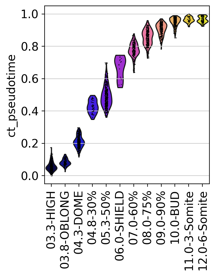
As expected, the CytoTRACE pseudotime increases for later time points. Thus, we can use this score to bias graph edges into the direction of increasing differentiation status, similar to how we do this for other pseudotimes with the PseudotimeKernel.

Compute & visualize a transition matrix

Compute the transition matrix using compute_transition_matrix().

ctk.compute_transition_matrix(threshold_scheme="soft", nu=0.5)

INFO     Computing transition matrix based on pseudotime                                                           

INFO         Finish (0.51s)                                                                                        

CytoTRACEKernel[n=2434, dnorm=False, scheme='soft', b=10.0, nu=0.5]

To get some intuition for this transition matrix, we can project it into an embedding and draw streamlines - the following plot will look like the plots you’re used to from scVelo and velocyto for visualizing RNA velocity [Bergen et al., 2020, La Manno et al., 2018].

Note

There’s no RNA velocity here, we’re visualizing the directed transition matrix we computed using the kNN graph as well as the CytoTRACE pseudotime.

ctk.plot_projection(basis="force_directed", color="Stage", legend_loc="right")

INFO     Projecting transition matrix onto 'force_directed'                                                        
INFO     Adding `adata.obsm['T_fwd_force_directed']` (0.19s)                                                       

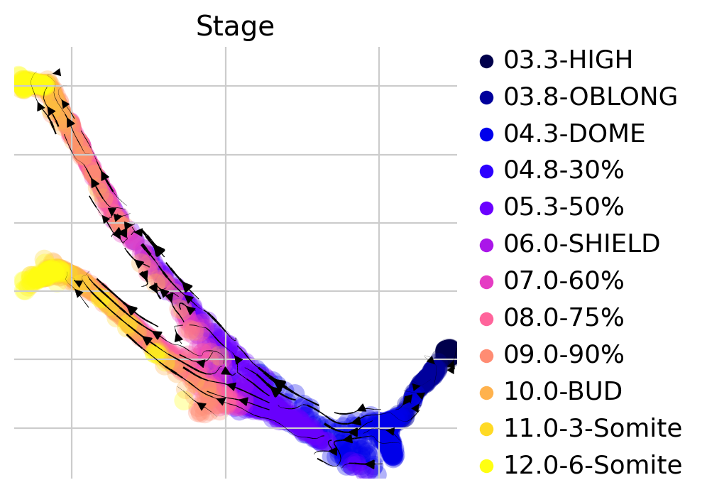
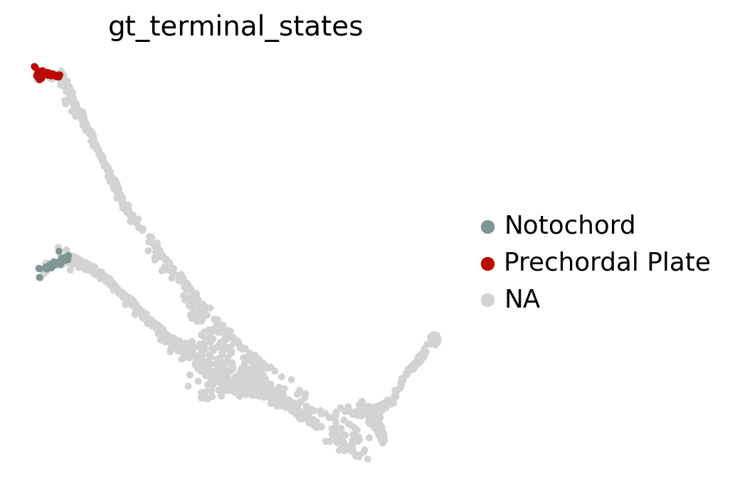
Visually, in the low-dimensional space, the process of differentiation seems to be captured well by this transition matrix. We can visually “confirm” this by looking at terminal-state annotations from the original study:

sc.pl.embedding(adata, basis="force_directed", color="gt_terminal_states")

Another way to gain intuition for the transition matrix is by drawing some cells from the early stage and to use these as starting cells to simulate random walks on the transition matrix. This visualization technique is less biased by the low-dimensional embedding as the random walks are computed directly based on the transition matrix.

ctk.plot_random_walks(
    n_sims=100,
    start_ixs={"Stage": "03.3-HIGH"},
    basis="force_directed",
    color="Stage",
    legend_loc="right",
    seed=1,
)

INFO     Simulating 100 random walks of maximum length 609                                                         

INFO         Finish (3.39s)                                                                                        
INFO     Plotting random walks                                                                                     

[0]PETSC ERROR: ------------------------------------------------------------------------
[0]PETSC ERROR: Caught signal number 13 Broken Pipe: Likely while reading or writing to a socket
[0]PETSC ERROR: Try option -start_in_debugger or -on_error_attach_debugger
[0]PETSC ERROR: or see https://petsc.org/release/faq/#valgrind and https://petsc.org/release/faq/
[0]PETSC ERROR: configure using --with-debugging=yes, recompile, link, and run 
[0]PETSC ERROR: to get more information on the crash.

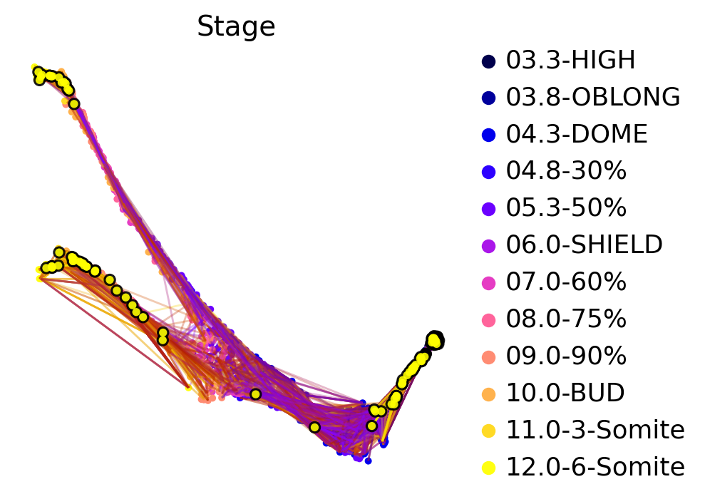
Black dots denote sampled starting cells for random walks, yellow dots denote end cells. We terminated each random walk after a predefined number of steps. Random walks are colored according to how long they’ve been running for - i.e. the initial segments are more black/blue whereas the late segments are more orange/yellow. We can see that many random walks terminate in one of the two terminal states, as expected. Quite a few of them seem to get stuck early on, this could be further investigated.

Note

The visualization techniques demonstrated here work for every kernel, no matter whether it’s a VelocityKernel, PseudotimeKernel, CytoTRACEKernel or some other CellRank kernel.

Closing matters

What’s next?

In this tutorial, you learned how to use CellRank to compute a transition matrix based on the CytoTRACE pseudotime and how it can be visualized in low dimensions. The real power of CellRank comes in when you use estimators to analyze the transition matrix directly, rather than projecting it. For the next steps, we recommend to:

• go through the initial and terminal states tutorial to learn how to use the transition matrix to automatically identify initial and terminal states.

• take a look at the API to learn about parameter values you can use to adapt these computations to your data.

• read the original CytoTRACE publication and considering limitations of this appraoch [Gulati et al., 2020].

Package versions

session_info2.session_info()