CellRank Meets RNA Velocity¶

Preliminaries¶

In this tutorial, you will learn how to:

use scvelo to compute RNA velocity [Bergen et al., 2020, La Manno et al., 2018].
set up CellRank’s VelocityKernel and compute a transition matrix based on RNA velocity.
combine the VelocityKernel with the ConnectivityKernel to emphasize gene expression similarity.
visualize the transition matrix in a low-dimensional embedding.

This tutorial notebook can be downloaded using the following link.

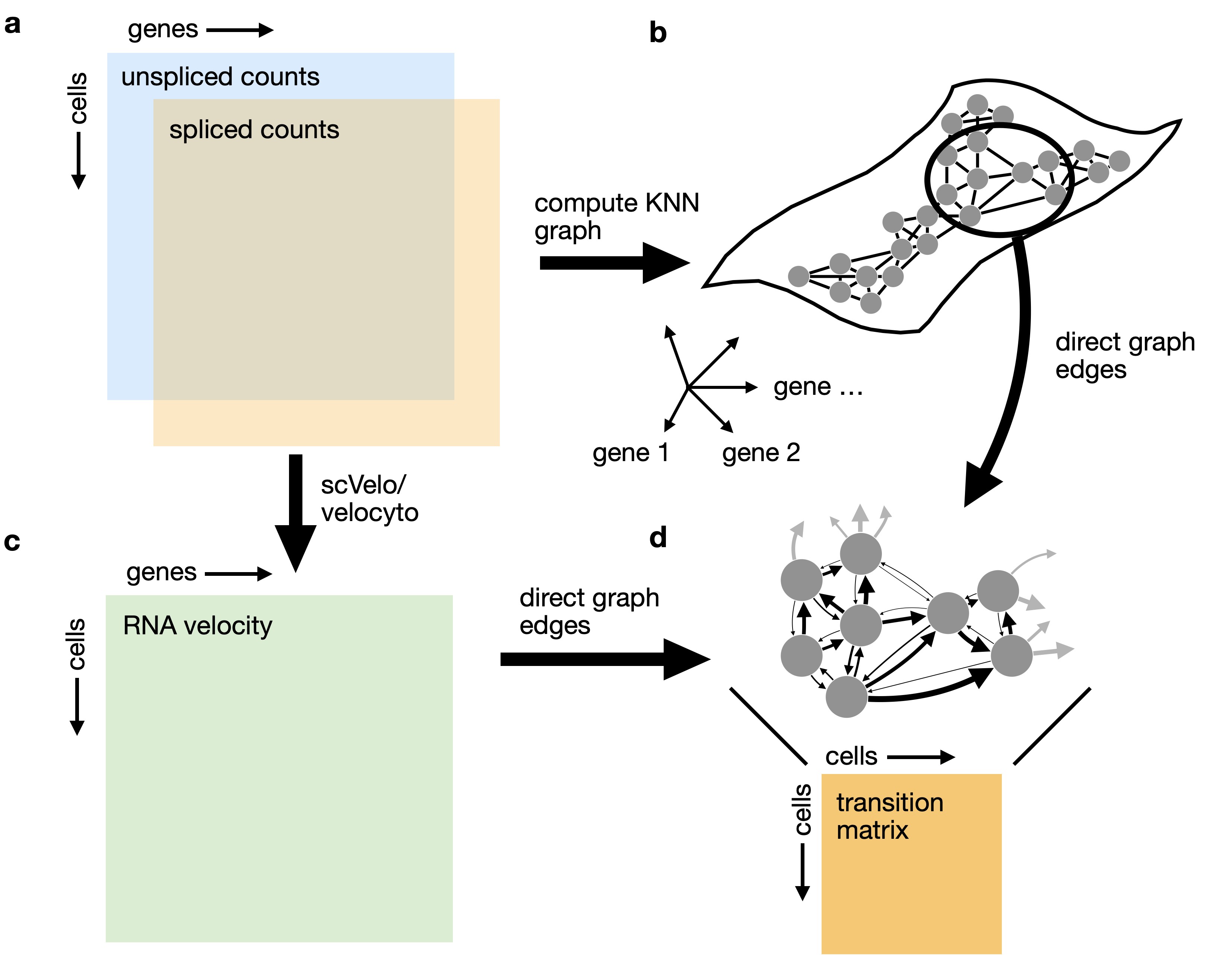
The VelocityKernel restricts velocity vectors to their local neighborhood to estimate a transition matrix. — **Using RNA velocity in high dimensions to analyze cellular transitions:** We combine RNA velocity with transcriptomic similarity in high dimensions to compute a matrix of cell-cell transition probabilities.¶

Note

If you want to run this on your own data, you will need:

a scRNA-seq dataset which has been preprocessed to contain unspliced & spliced counts using a software like the Velocyto command line tool.

Note

If you encounter any bugs in the code, our if you have suggestions for new features, please open an issue. If you have a general question or something you would like to discuss with us, please post on the scverse discourse.

Import packages & data¶

%load_ext autoreload
%autoreload 2

import sys

if "google.colab" in sys.modules:
    !pip install -q git+https://github.com/scverse/cellrank

import cellrank as cr
import scanpy as sc
import scvelo as scv
import session_info2

scv.settings.verbosity = 3
cr.settings.logging_level = "INFO"

import warnings

warnings.simplefilter("ignore", category=UserWarning)

To demonstrate the appproach in this tutorial, we will use a scRNA-seq dataset of mouse pancreas development at embryonic day (E) 15.5, which can be conveniently acessed through pancreas [Bastidas-Ponce et al., 2019, Bergen et al., 2020].

We visualize the fraction of spliced/unspliced reads; these are required to estimate RNA velocity.

adata = cr.datasets.pancreas()
scv.pl.proportions(adata)
adata

../../../_images/f5e84c7e8bb146c556559fe816a4c63561b6e3fbf5ee824c0241d9cc2a61c82c.png

AnnData object with n_obs × n_vars = 2531 × 27998
    obs: 'day', 'proliferation', 'G2M_score', 'S_score', 'phase', 'clusters_coarse', 'clusters', 'clusters_fine', 'louvain_Alpha', 'louvain_Beta', 'palantir_pseudotime'
    var: 'highly_variable_genes'
    uns: 'clusters_colors', 'clusters_fine_colors', 'day_colors', 'louvain_Alpha_colors', 'louvain_Beta_colors', 'neighbors', 'pca'
    obsm: 'X_pca', 'X_umap'
    layers: 'spliced', 'unspliced'
    obsp: 'connectivities', 'distances'

Preprocess the data¶

Filter out genes which don’t have enough spliced/unspliced counts, normalize and log transform the data and restrict to the top highly variable genes. Further, compute principal components and moments for velocity estimation.

# filter and normalize - scVelo uses pre-filtering gene counts per cell to determine
# the library size for normalization
scv.pp.filter_genes(adata, min_shared_counts=20)
scv.pp.normalize_per_cell(adata)

# log transformation and hvg
sc.pp.log1p(adata)
sc.pp.highly_variable_genes(adata, n_top_genes=2000)

# pca, neighbors, and moments.
sc.tl.pca(adata)
sc.pp.neighbors(adata, n_pcs=30, n_neighbors=30, random_state=0)
scv.pp.moments(adata, n_pcs=None, n_neighbors=None)

Filtered out 22024 genes that are detected 20 counts (shared).
Normalized count data: X, spliced, unspliced.
computing moments based on connectivities
    finished (0:00:00) --> added 
    'Ms' and 'Mu', moments of un/spliced abundances (adata.layers)

Run scVelo¶

We will use scVelo’s dynamical model to estimate model parameters.

Note

Please make sure to have at least version 0.2.3 of scVelo installed to make use parallelisation in scv.tl.recover_dynamics. On my MacBook, using 8 cores, the below cell takes about 1 min to execute.

scv.tl.recover_dynamics(adata, n_jobs=8)

recovering dynamics (using 8/128 cores)

/cluster/project/treutlein/USERS/mlange/github/cellrank/docs/notebooks/.pixi/envs/default/lib/python3.12/multiprocessing/popen_fork.py:66: DeprecationWarning: This process (pid=563875) is multi-threaded, use of fork() may lead to deadlocks in the child.
  self.pid = os.fork()

    finished (0:00:35) --> added 
    'fit_pars', fitted parameters for splicing dynamics (adata.var)

Once we have the parameters, we can use these to compute the actual velocities.

scv.tl.velocity(adata, mode="dynamical")

computing velocities
    finished (0:00:00) --> added 
    'velocity', velocity vectors for each individual cell (adata.layers)

We’ll use CellRank to visualize the velocities in an embedding further down below.

Combine RNA velocity with expression similarity in high dimensions¶

Set up the VelocityKernel¶

Set up the VelocityKernel from the AnnData object containing the scVelo-computed velocities.

vk = cr.kernels.VelocityKernel(adata)

Use the VelocityKernel to compute a transition matrix by correlating each cell’s velocity vector with the displacement vectors towards nearest neighbors, directly in high-dimensional gene expression space.

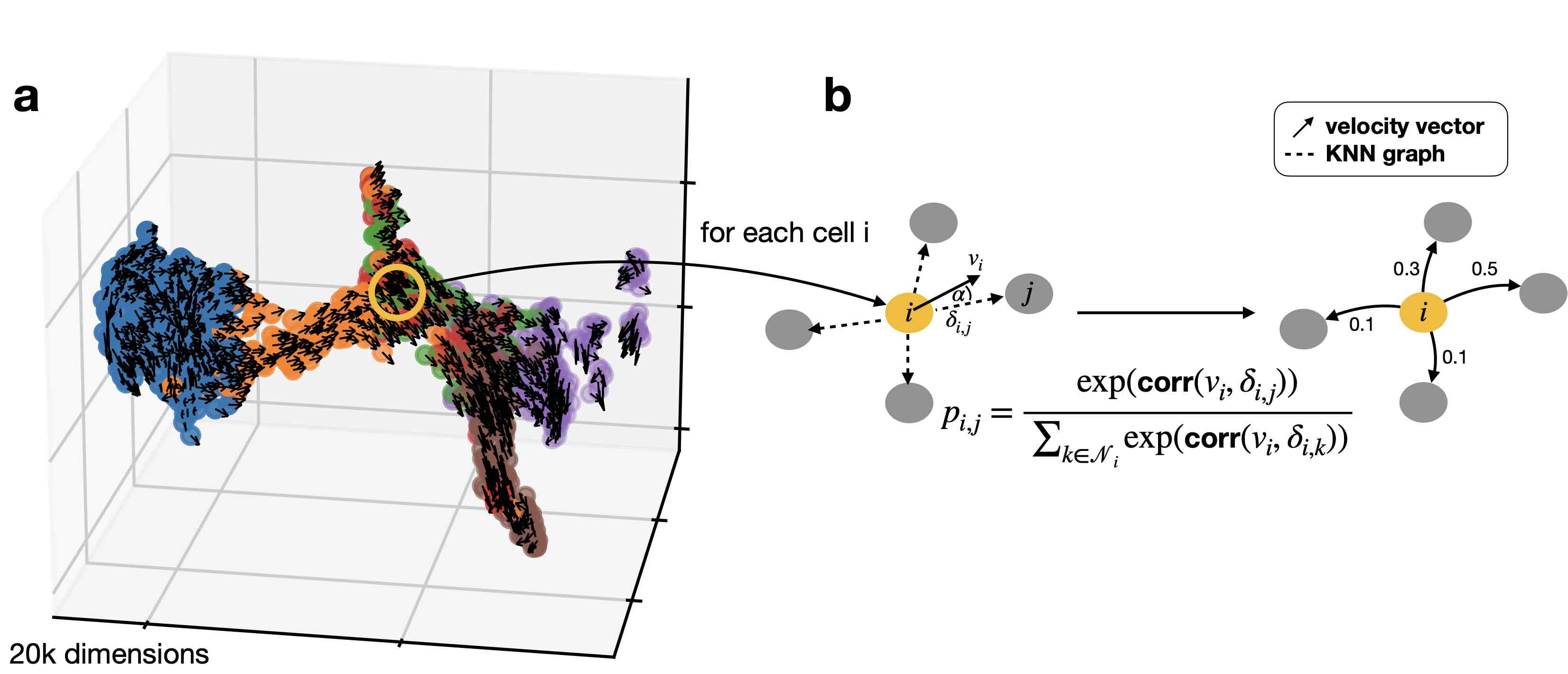
Correlating velocity vectors with transcriptomic displacements gives sparse transition probabilities. — **Computing transition probabilities:** We correlate each cell’s velocity vector with the transcriptomic displacement vectors towards nearest neighbors.¶

We do this using the compute_transition_matrix() method.

vk.compute_transition_matrix()

INFO     Computing transition matrix using 'deterministic' model

/cluster/project/treutlein/USERS/mlange/github/cellrank/docs/notebooks/.pixi/envs/default/lib/python3.12/multiprocessing/popen_fork.py:66: DeprecationWarning: This process (pid=563875) is multi-threaded, use of fork() may lead to deadlocks in the child.
  self.pid = os.fork()

INFO     Using `softmax_scale=3.9731`

/cluster/project/treutlein/USERS/mlange/github/cellrank/docs/notebooks/.pixi/envs/default/lib/python3.12/multiprocessing/popen_fork.py:66: DeprecationWarning: This process (pid=563875) is multi-threaded, use of fork() may lead to deadlocks in the child.
  self.pid = os.fork()

INFO         Finish (8.88s)

VelocityKernel[n=2531, model='deterministic', similarity='correlation', softmax_scale=np.float64(3.973)]

By default, we use the deterministic mode to compute the transiton matrix. If you want to propagate uncertainty in the velocity vectors, check out the stochastic and monte_carlo modes. The stochastic mode estimates a distribution over velocity vectors using the KNN graph and propagates this distribution into the transition matrix using an analytical approximation.

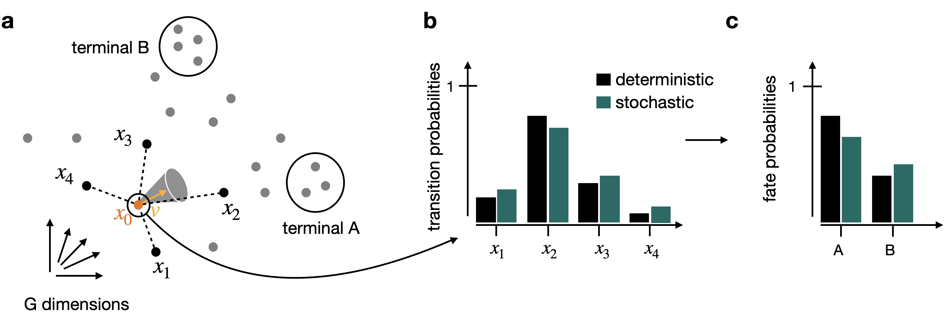
Propagating uncertainty from velocity vectors into cell state transitions. — **Propagating velocity uncertainty:** CellRank can propagate estimated velocity uncertainties into transition probabilities.¶

Note

Please check out our “CellRank for directed single-cell fate mapping” paper to learn more on uncertainty propagation and how it makes computations more robust to noise [Lange et al., 2022].

Combine with gene expression similarity¶

RNA velocity can be a very noise quantity; to make our computations more robust, we combine the VelocityKernel with the similarity-based ConnectivityKernel.

ck = cr.kernels.ConnectivityKernel(adata)
ck.compute_transition_matrix()

combined_kernel = 0.8 * vk + 0.2 * ck

INFO     Computing transition matrix based on adata.obsp['connectivities']                                         
INFO         Finish (0.01s)                                                                                        

Above, we combined the two kernels with custom weights given to each. The same syntax can be used to combine any number of CellRank kernels, see the getting started tutorial.

Let’s print the combined kernel object to see what it contains:

print(combined_kernel)

(0.8 * VelocityKernel[n=2531] + 0.2 * ConnectivityKernel[n=2531])

This tells us about the kernels we combined, the weights we used to combine them, and the parameters that went into transition matrix computation for each kernel. Check out the API to learn more about the parameters. Next, let’s explore ways to visualize the computed transition matrix.

Visualize the transition matrix¶

Similar to scvelo [Bergen et al., 2020] and velocyto [La Manno et al., 2018], CellRank visualizes the transition matrix in any low dimensional embedding (UMAP, t-SNE, PCA, Diffmap, etc.) via arrows or streamlines.

vk.plot_projection()

INFO     Projecting transition matrix onto 'umap'                                                                  
INFO     Adding `adata.obsm['T_fwd_umap']` (0.27s)                                                                 

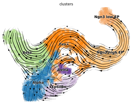
../../../_images/52675a3f79560720bce802067fdf37fe1393d5c5860f15190797e2f0baac3148.png

As shown before in the scVelo publication [Bergen et al., 2020], the projected velocity vectors capture the overall trend in this system: Neurogenin 3 low endocrine progenitor cells (Ngn3 low EP) gradually transition via indermediate stages towards terminal, hormone producing Alpha, Beta, Epsilon and Delta cells. Another way to visualize this is via random walks.

vk.plot_random_walks(
    start_ixs={"clusters": "Ngn3 low EP"},
    max_iter=200,
    seed=0,
    legend_loc="on data",
    color="clusters",
)

INFO     Simulating 100 random walks of maximum length 200

/cluster/project/treutlein/USERS/mlange/github/cellrank/docs/notebooks/.pixi/envs/default/lib/python3.12/multiprocessing/popen_fork.py:66: DeprecationWarning: This process (pid=563875) is multi-threaded, use of fork() may lead to deadlocks in the child.
  self.pid = os.fork()

INFO         Finish (1.49s)                                                                                        
INFO     Plotting random walks                                                                                     

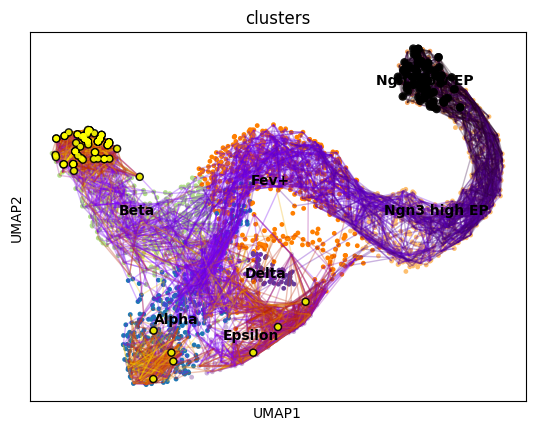
../../../_images/46dc567ee894d804281bf1eb0babeec8492322d4aa2aacdc25edbf77051d3153.png

We simulated random walks starting in the Ngn3 low EP cluster. Black and yellow dots denote the start and end points of a random walk, respectively. In agreement with known biology, the Beta cluster is dominant at E15.5 [Bastidas-Ponce et al., 2019].

Note

Take these low-dimensional representations with a grain of salt; streamlines in a low-dimensional embeddings are very biased by the topology of that embedding. They often oversmooth that actual dynamics, or obscure them entirely. Random walks are a better alternative; these are sampled directly from the Markov chain and don’t depend on the low dimensional embedding. Additionally, we recommend analyzing high-dimensional dynamics using estimators.

Closing matters¶

Write results to file¶

We will use the kernel computed here in other tutorials to demonstrate downstream applications. For this reason, we write the kernel attributes to the underlying anndata.AnnData object here and save to disk. In other tutorials, we can then reconstruct the kernel from the saved object. The dataset written here is available via cellrank.datasets.pancreas by specifying kind="preprocessed-kernel".

vk.write_to_adata()
adata.write(
    "datasets/endocrinogenesis_day15.5_velocity_kernel.h5ad", compression="gzip"
)

What’s next?¶

In this tutorial, you learned how to use CellRank to compute a transition matrix using RNA velocity and gene expression similarity and how it can be visualized in low dimensions [Bergen et al., 2020, La Manno et al., 2018, Lange et al., 2022]. The real power of CellRank comes in when you use estimators to analyze the transition matrix directly, rather than projecting it. For the next steps, we recommend…

going through the initial and terminal states tutorial to learn how to use the transition matrix to automatically identify initial and terminal states.
reading our “CellRank for directed single-cell fate mapping” paper to learn more about the methods we used here [Lange et al., 2022].
taking a look at the API to learn about parameter values you can use to adapt these computations to your data.

Package versions¶

We used the following package versions to generate this tutorial:

session_info2.session_info()